XB-IMG-176011
Xenbase Image ID: 176011
|
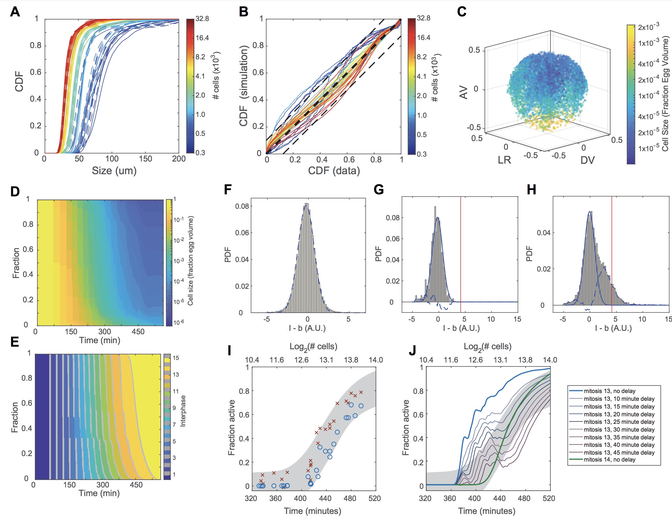
Figure S5. Validation of Computational Model for Zygotic Genome Activation. Related to Figure 5. (A-J).
(A) Cumulative distribution functions (CDFs) of cell sizes of 40 measured embryos (solid lines) and simulated embryos
(dashed lines) with the same number of cells.
(B) Comparison of simulated (y axis) and measured (x axis) CDF values at all cell sizes. Perfect correspondence indicated by thick dashed line with slope equal to unity. Thin dashed lines indicate 12.5% deviation from unity. AKA the line of
identity. Colors in A and B indicate number of cells.
(C) Spatial distribution of cell sizes in a single representative simulated embryo. AV, animal-vegetal axis; LR, left-right
axis; DV, dorsal-ventral axis.
(D) Distribution of cell sizes as a function of time for 100 simulated embryos.
(E) Distribution of mitotic cycles as a function of time for 100 simulated embryos.
(F-H) Estimation of confidence intervals for the fraction of active cells. Lower limit of active fraction is estimated using a
global EU intensity threshold (red vertical lines in G, H) as described in Methods. Upper limit is estimated by assuming
a common distribution of background-subtracted fluorescence intensity values for inactive cells. PDF, probability density
function.
(F) Distribution of nonspecific fluorescence was determined by computing the background-subtracted EU intensity distri- bution for 18 young embryos prior to ZGA and containing between 464 and 3357 cells. The distribution was fit to a
normal distribution (dashed blue line, mu = -0.24, sigma = 1.09). Subtracting a rescaled normal distribution with this
width yielded the distribution of EU intensities corresponding to active nuclei.
(G) The rescaled normal distribution (solid blue line) does not perfectly describe the distribution from an individual
young, inactive embryo (this example: 664 cells). Subtracting the idealized normal distribution from the actual distribu- tion (dashed blue line) yields an estimate of error in the upper limit of the confidence interval. The average error across
18 embryos is 3% as calculated by summing the total area between the dashed line and the x axis.
(H) Applying the same procedure to an embryo undergoing ZGA provides an estimate of the fraction of cells that do not
exceed the global threshold but whose intensities are found with greater frequency than expected in an inactive embryo.
The embryo shown contains 7496 cells. The upper and lower bounds on the fraction of active cells for this embryo are
12% and 44%.
(I) For each embryo, the upper (red x) and lower (blue o) limits of the fraction of active cells are plotted. A logistic function
was then fit to the set of upper or lower limits across all 40 embryos to generate the confidence interval (gray shaded
band). The confidence interval, which contains 95% of all observations, represents the upper and lower logistic functions
plus (or minus) 6%. These data points and confidence intervals are used in Figure 4.
(J) Comparison of counter model implemented with detectable genome activation following mitosis 14 (green), following
mitosis 13 with no delay in detection (blue), or with increasing duration of delay until the accumulation of detectable
signal. Activation at cycle 13 followed by a delay of 30 minutes falls largely within the confidence interval. Image published in: Chen H et al. (2019) Copyright © 2019. Image reproduced with permission of the Publisher, Elsevier B. V. Larger Image Printer Friendly View |