Xenbase Image ID: 122634

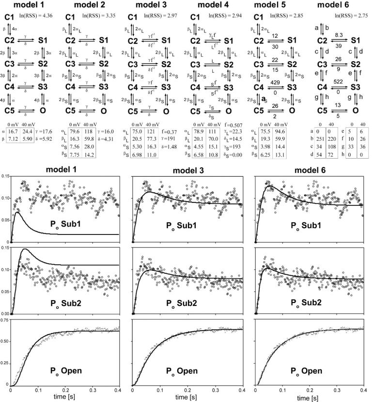
Figure 12. Subunit-subconductance models. To investigate whether the subunit-subconductance model can accurately describe the single channel behavior of the S-L dimer, Markov models were generated that represent specific instances of the general model shown in Fig. 5 B. The six extremely short-lived sublevels, which have a gray background in Fig. 5 B, were omitted from the Markov models, since the majority of visits to these levels will go undetected due to the low pass filtering. This results in nine resolvable states: five closed states (C1–C5), three sublevels (S1–S3), and the open state (O). Six variations were used (models 1–6) for which the number of free (optimized) parameters increases with the model, by reducing the number of constraints. Each Markov scheme defines a set of nine differential equations that were integrated to generate models of Po(t), FL(t), and COP(t) for Sub1, Sub2, and Open, at 0 and +40 mV (a total of 18 curves). Activation rate constants (vertical transitions) depend on membrane potential; rate constants describing channel opening (horizontal transitions) are voltage independent. For the Po(t) and FL(t) curves, it was assumed that all channels are in C1 at t = 0. The initial conditions for the COP(t) curves are not known and were therefore estimated. There are nine Markov states for three COP curves (Sub1, Sub2, Open) at two membrane potentials, resulting in 54 initial conditions to be estimated. In addition, rate constants and allosteric factors were estimated for each model by minimizing the sum of squared residuals (RSS) between the data and the model using the Solver in Microsoft Excel. Optimized values are provided for each model. The natural log of the residual sum of squares (RSS) is shown for each model as a relative measure of goodness-of-fit. Model 1 is the most severely constrained model and it makes two assumptions: (1) that there are four identical and independent voltage sensors, and (2) that opening transitions do not depend on the number of activated subunits. These constraints result in a model with only six free rate constants. The model provided a very poor description of the data, as illustrated by the Po(t) curve fits below. Model 2 takes into account that the S-L dimer contains subunits with distinct voltage sensors. Activation is described by two fast L sensors and two slower S sensors. Voltage sensors still move independently, and opening transitions do not depend on the number of activated subunits. This model has 10 free rate constants. Model 3 improves upon model 2 by introducing an allosteric factor (f) that allows opening efficiency to depend on the number of activated subunits. Although the number of parameters increases by only 1, the goodness-of-fit increases significantly, as shown by the Po(t) curve fits below. Model 4 allows the opening transitions to be different for the L and S subunit, while they share a single allosteric factor. This results in a small increase in the goodness-of-fit. Model 5 removes all constraints from the opening (horizontal) transitions and incrementally improves the fit. In model 6, all constraints are removed, resulting in 24 free rate constants. This last model has the smallest value of ln(RSS), consistent with it having the least number of constraints. However, the improvements made by models 4–6 over model 3 are only incremental (1%), compared with the substantial reductions in ln(RSS) made by models 2 and 3, (23% and 11%, respectively). Image published in: Chapman ML and VanDongen AM (2005) Copyright © 2005, The Rockefeller University Press. Creative Commons Attribution-NonCommercial-ShareAlike license Larger Image Printer Friendly View

Return to previous page